Data Set Description¶

The “Tyrolean” data set provides hourly observations from two stations, namely “Ellbögen” and “Sattelberg” located in Tyrol, Austria.

Ellbögen is our target station (valley site) located in the Wipp Valley, a north-south oriented alpine valley on the northern side of the European Alps. To the north the Wipp Valley opens into the Inn Valley (close to Innsbruck, the capitol of Tyrol), to the south the valley ends at a narrow gap in the main Alpine ridge called Brennerpass (\(1370~m\); the pass between Austria and Italy) flanked by mountains (\(>2100~m\)). The Wipp Valley is one of the lowest and most distinct cuts trough the Alpine mountain range and well known for south foehn (north of the Alps). Station Sattelberg serves as crest station and provides observations of the upstream air mass during south foehn events. The station is located on top of the mountain to the west of the pass.

Loading the Data Set¶

The call foehnix.get_demodata('tyrol') returns the combined data set for both station (Ellbögen and Sattelberg). In addition, the potential temperature difference between the two stations is calculated by reducing the dry air temperature from “Sattelberg” to the height of “Ellbögen” (dry adiabatic lapse rate of 1K per 100m; stored on diff_t). Details can be found on the get_demodata() reference page.

In [1]: import numpy as np

In [2]: import foehnix

# load the data for Tyrol and show a summary:
In [3]: data = foehnix.get_demodata('tyrol')

In [4]: data.head()
Out[4]: 
                      timestamp     dd   ff     rh    t  dd_crest  ff_crest  rh_crest  t_crest  diff_t
timestamp                                                                                             
2006-01-01 01:00:00  1136077200  171.0  0.6   90.0 -0.4     180.0      10.8     100.0     -7.8    2.87
2006-01-01 02:00:00  1136080800  268.0  0.3  100.0 -1.8     186.0      12.5     100.0     -8.0    4.07
2006-01-01 03:00:00  1136084400  115.0  5.2   79.0  0.9     181.0      11.3     100.0     -7.4    1.97
2006-01-01 04:00:00  1136088000  152.0  2.1   88.0 -0.6     178.0      13.3     100.0     -7.5    3.37
2006-01-01 05:00:00  1136091600  319.0  0.7  100.0 -2.6     176.0      13.1     100.0     -7.1    5.77

The data set returned is a regular pandas.DataFrame object. Note that the data set is not strictly regular (contains hourly observations, but some are missing) and contains quite some missing values (NaN). This is not a problem as the functions and methods will take care of missing values and inflate the time series object (regular \(\rightarrow\) strictly regular).

Important: The names of the variables in the Tyrolean data set are the “standard names” on which most functions and methods provided by this package are based on. To be precise:

• Valley station: air temperature t, relative humidity rh, wind speed ff, wind direction dd (meteorological, degrees \(\in [0, 360]\))
• Crest station: air temperature t_crest, relative humidity rh_crest, wind speed ff_crest, wind direction dd_crest (\(\in [0, 360]\))
• Note: The crest station syntax is different from the R foehnix version, where a prefix is used (e.g. crest_ff).
• In addition: Potential temperature difference diff_t (calculated by get_demodata())

… however, all functions have arguments which allow to set custom names (see “[Demos > Viejas (California, USA)](articles/viejas.html)” or function references).

Based on prior knowledge we define two “foehn wind sectors” as follows:

• At Ellbögen the observed wind direction (dd) needs to be along valley within 43 and 223 degrees (south-easterly; a 180 degree sector).
• At Sattelberg the observed wind direction (dd_crest) needs to be within 90 and 270 degrees (south wind; 180 degree sector).

Estimate Classification Model¶

The most important step is to estimate the foehnix.Foehnix classification model. We use the following model assumptions:

• Main variable: diff_t is used as the main covariate to separate ‘foehn’ from ‘no foehn’ events (potential temperature difference).
• Concomitant variable: rh and ff at valley site (relative humidity and wind speed).
• Wind filters: two filters are defined. dd = [43, 223] for Ellbögen and dd_crest = [90, 270] for Sattelberg (see above).
• Option switch: switch=True as high diff_temp indicate stable stratification (no foehn).

Run the model and show a summary

# Estimate the foehnix classification model
In [5]: tyrol_filter = {'dd': [43, 223], 'dd_crest': [90, 270]}

In [6]: model = foehnix.Foehnix('diff_t', data, concomitant=['rh', 'ff'], filter_method=tyrol_filter, switch=True)

In [7]: model.summary(detailed=True)

Number of observations (total)   113952 (5527 due to inflation)
Removed due to missing values     38859 (34.1 percent)
Outside defined wind sector       50665 (44.5 percent)
Used for classification           24428 (21.4 percent)

Climatological foehn occurance 18.36 percent (on n = 75093)
Mean foehn probability 18.06 percent (on n = 75093)

Log-likelihood: -55044.0, 7 effective degrees of freedom
Corresponding AIC = 110101.9, BIC = 110158.6

Number of EM iterations 5/100 (converged)
Time required for model estimation: 0.6 seconds

------------------------------------------------------

Components: t test of coefficients

               Estimate  Std. Error     t_value  Pr(>|t|)
(Intercept).1  5.799082    0.024419  237.485686       0.0
(Intercept).2  0.858603    0.010773   79.697585       0.0

------------------------------------------------------

Concomitant model: z test of coefficients

              Estimate  Std. Error     z_value      Pr(>|z|)
cc.Intercept  0.812719    0.105710    7.688184  1.492381e-14
cc.rh        -1.029320    0.001446 -711.848118  0.000000e+00
cc.ff         3.305431    0.012133  272.422207  0.000000e+00

Number of IWLS iterations 3 (converged)
Dispersion parameter for binomial family taken to be 1.

In [8]: model.coef['mu1']
Out[8]: 5.7990815368565505

In [9]: np.exp(model.coef['logsd1'])
Out[9]: 2.6406847321165876

In [10]: model.coef['mu2']
Out[10]: 0.8586032145482315

In [11]: np.exp(model.coef['logsd2'])
Out[11]: 1.328458443236942

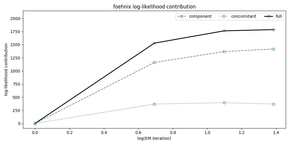
Graphical Model Assessment¶

A Foehnix object comes with generic plots for graphical model assessment.

The following figure shows the ‘log-likelihood contribution’ of

• the main component (left hand side of formula),
• the concomitant model (right hand side of formula),
• and the full log-likelihood sum which is maximised by the optimization algorithm.

The abscissa shows (by default) the logarithm of the iterations during optimization.

In [12]: model.plot('loglikcontribution', log=True)

In addition, the coefficient paths during optimization can be visualized:

In [13]: model.plot('coef', log=True)

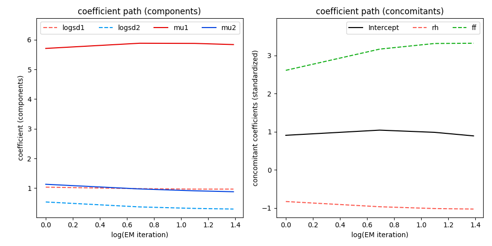
The left plot shows the parameters of the two components (\(\mu_1, \log(\sigma_1), \mu_2, \log(\sigma_2)\)), the right one the standardized coefficients of the concomitant model.

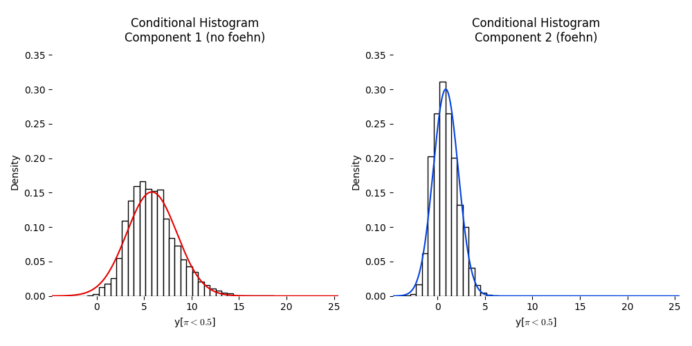
Last but not least a histogram with the two clusters is plotted. 'hist creates an empirical density histogram separating “no foehn” and “foehn” events adding the estimated distribution for these two clusters.

In [14]: model.plot('hist')

Time Series Plot¶

In [15]: model.plot('timeseries', start='2017-02-01', end='2017-02-11', ndays=11)

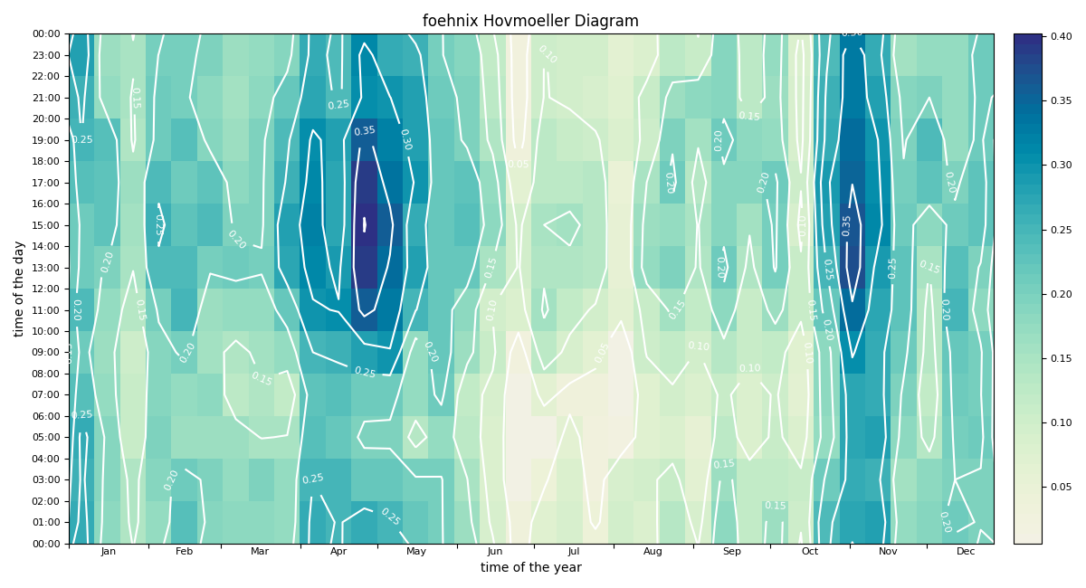
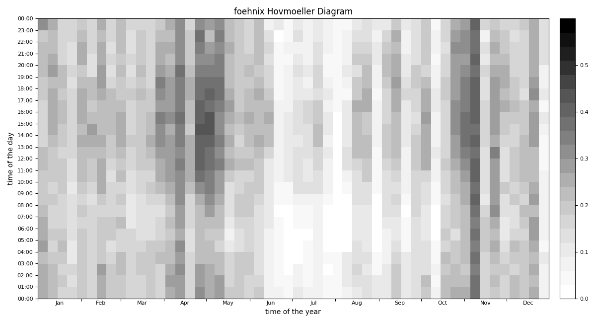
Hovmoeller Diagram¶

The image function plots a Hovmoeller Diagram to assess foehn freqency

In [16]: model.plot('image', deltat=3600, deltad=7)

Customized plot which shows the “foehn frequency” with custom colors and additional contour lines and custom aggregation period (10-days, 3-hourly).

In [17]: import colorspace

In [18]: mycmap = colorspace.sequential_hcl(palette='Blue-Yellow', rev=True).cmap(51)

In [19]: model.plot('image', deltat=2*3600, deltad=10, cmap=mycmap,
   ....:            contours=True, contour_color='w', contour_levels=np.arange(0, 1, 0.05),
   ....:            contour_labels=True)
   ....: